Biological Delay Dynamics and Time Delay
In neurobiology, it is well documented that neurons do not process incoming information instantaneously. Instead, they integrate incoming electrical signals into their membrane potential over time. Only when this membrane potential exceeds a critical threshold does the cell fire an action potential (spike). Consequently, the temporal dimension plays a decisive role: both the timing and arrival order of incoming signals directly influence neuronal activation.
Inspired by this biological mechanism, we can build not only time-dependent and coupled partial neural networks, but also incorporate explicit time delays (\(\tau\)). Embedding delays into partial differential equations – leading to partial delay differential equations (Delay PDEs) – is an established concept in mathematical modeling and frequently occurs in real biological and physical systems.
Example: PNN with Time Delay (Spike)
System for \(u\) (Neuron \(h_1\) with delay \(\tau\))
$$\begin{cases}
\frac{\partial \sigma(u(t+\tau))}{\partial u} = \sigma(u)\bigl(1 - \sigma(u)\bigr) \\[1.5ex]
\nabla u = \mathbf{m}_1 \\[1ex]
u(0) = u_0 \\[1ex]
\frac{\partial u}{\partial t} = c_0
\end{cases}$$
System for \(v\) (Neuron \(h_2\))
$$\begin{cases}
\frac{\partial \sigma(v)}{\partial v} = \sigma(v)\bigl(1 - \sigma(v)\bigr) \\[1.5ex]
\nabla v = \mathbf{m}_2 \\[1ex]
v(0) = v_0 \\[1ex]
\frac{\partial v}{\partial t} = c_1
\end{cases}$$
In this formulation, the parameter $\tau$ represents the characteristic time delay (lag). While $\tau$ can be derived analytically or fixed based on domain-specific PDE dynamics, it can also be treated as a continuous, learnable parameter.
Learnable and Adaptive Activation Functions in PNNs
At this point, we emphasize that the underlying partial differential equation for the activation function does not need to be fixed a priori. Instead, the network can dynamically adjust its activation behavior during optimization or learn an entirely new activation function over time to better describe the underlying system.
Example: PNN with Dynamic / Adaptive Activation Function
System for \(u\) (Neuron \(h_1\) with learnable mixing parameter \(\alpha\))
$$\begin{cases}
\frac{\partial \sigma}{\partial u} = (1 - \alpha) \, \sigma(u)\bigl(1 - \sigma(u)\bigr) + \alpha \, \Theta(u) \\[1.5ex]
\nabla u = \mathbf{m}_1 \\[1ex]
u(0) = u_0(x) \\[1ex]
\frac{\partial u}{\partial t} = c_0
\end{cases}$$
In this setup, \(\alpha \in [0, 1]\) acts as a learnable interpolation parameter, and \(\Theta(u)\) represents the Heaviside step function—whose direct integration yields the Rectified Linear Unit (ReLU), since \(\int \Theta(u) \, du = \max(0, u) = \text{ReLU}(u)\). Through optimization, the network adaptively determines which activation characteristics are best suited for the system. Specifically, when \(\alpha = 0\), the activation derivative reduces strictly to the standard sigmoid formulation, whereas \(\alpha = 1\) shifts the dynamics to a ReLU-like response. During training, the framework can continuously refine or smoothly transition between these functional forms.
Remarks on Neural ODEs and Physics-Informed Neural Networks
At this point, we would like to offer a few remarks regarding the fields of Neural Ordinary Differential Equations (Neural ODEs) and Physics-Informed Neural Networks (PINNs). In general, these frameworks do not address partial neural networks; however, certain Neural ODEs or PINNs can be viewed as special, degenerate cases within this broader theory. Partial Neural Networks represent a higher-order generalization of standard neural architectures.
We hypothesize that the entire system of neurons in a partial neural network can be represented abstractly as an operator semigroup—specifically as a multi-parameter semigroup depending on multiple time variables, indexed by layer depth or introduced time intervals. To capture the complete state of the PNN, this semigroup must be evaluated at these specific time steps.
Formally, for independent time parameters \(t_1, t_2, \dots, t_n \ge 0\), the family of operators \(S(t_1, \dots, t_n)\) characterizes the global partial neural network by satisfying the semigroup property:
$$S(t + s) = S(t) S(s) \quad \text{for } t, s \in \mathbb{R}_+^n$$
The development of this mathematically rigorous operator-theoretic foundation remains an active direction for future research at the intersection of partial differential equations and functional analysis.
General Partial Neural Networks (PNN)
Definition: Partial Neural Network (PNN)
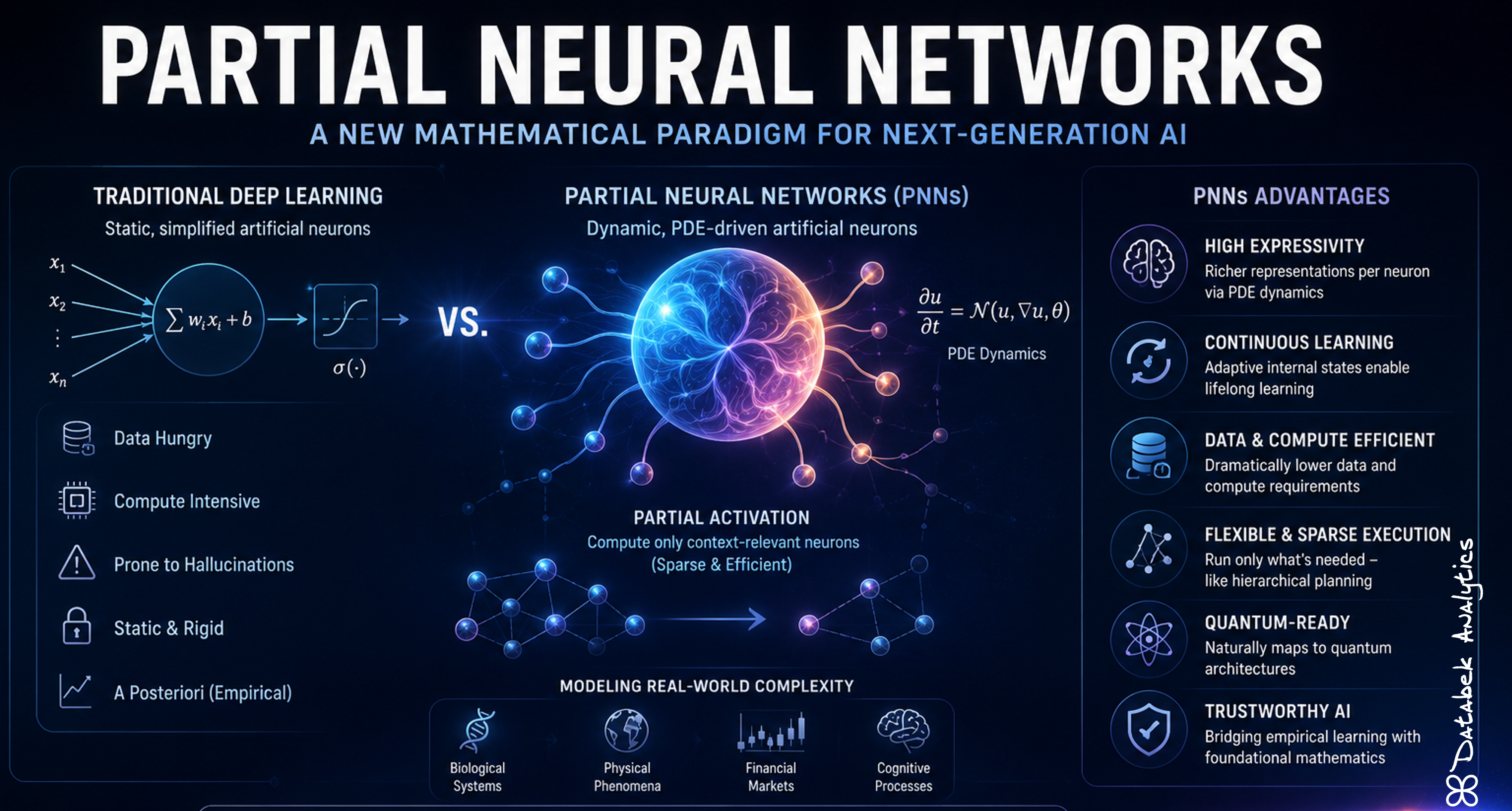
A Partial Neural Network (PNN) is an integrated architecture defined as a global system of non-linear, coupled, and time-dependent partial differential equations (PDEs). By mapping individual neurons and layer transitions to specific PDE boundary value problems, the entire network processes spatial features and temporal dynamics simultaneously as a unified dynamical system to model complex, high-dimensional phenomena.
Mathematical Formulation
Let \(\Omega \subset \mathbb{R}^d\) be a spatial domain and \(T > 0\) the time horizon. We consider a network with \(L\) hidden layers, where layer \(l \in \{1, \dots, L\}\) contains exactly \(N_l\) neurons, represented by the state vector \(\mathbf{u}^{(l)}(x, t) = \bigl(u_1^{(l)}(x, t), \dots, u_{N_l}^{(l)}(x, t)\bigr)^T \in \mathbb{R}^{N_l}\).
We define a Partial Neural Network as a system of coupled, non-linear partial differential equations of arbitrary order \(k \in \mathbb{N}\). The general system for layer \(l\) reads:
$$\begin{cases}
\mathcal{L}_{\psi}^{(l)}\left( \mathbf{u}^{(l)}, \frac{\partial \mathbf{u}^{(l)}}{\partial t}, \dots, \frac{\partial^{k_1} \mathbf{u}^{(l)}}{\partial t^{k_1}}, \nabla \mathbf{u}^{(l)}, \Delta \mathbf{u}^{(l)}, \dots \right) = \mathbf{F}^{(l)}\left(\mathbf{u}^{(l)}, \mathbf{u}^{(l-1)}, \mathbf{W}_{\psi}^{(l)}, t\right) \\[2.5ex]
\mathcal{L}_{x}^{(l)}\left( \mathbf{u}^{(l)}, D_x^{\alpha} \mathbf{u}^{(l)} \right) = \mathbf{M}^{(l)}\left(\mathbf{u}^{(l)}, \mathbf{u}^{(l-1)}\right) + \sum_{j=1}^{N_l} \mathbf{\alpha}_{j}^{(l)} \, g\left(D_x^{\beta} u_j^{(l)}\right) \\[2.5ex]
\mathcal{L}_{t}^{(l)}\left( \frac{\partial^{k_2} \mathbf{u}^{(l)}}{\partial t^{k_2}}, \dots, \frac{\partial \mathbf{u}^{(l)}}{\partial t}, \mathbf{u}^{(l)} \right) = \mathbf{C}^{(l)}(t) + \mathbf{H}^{(l)}\left(\mathbf{u}^{(l)}, \mathbf{u}^{(l-1)}, D_x^{\gamma} \mathbf{u}^{(l)}\right) \\[2.5ex]
\mathcal{B}\left( \mathbf{u}^{(l)}(x, t) \right) = \mathbf{g}^{(l)}(x, t) \quad \text{on } \partial\Omega \times [0, T] \quad \text{(Boundary Conditions)} \\[1.5ex]
\frac{\partial^m \mathbf{u}^{(l)}}{\partial t^m}(x, 0) = \mathbf{u}_{m, 0}^{(l)}(x) \quad \text{for } m = 0, \dots, k-1 \quad \text{(Initial Conditions)}
\end{cases}$$
Where:
- \(\mathcal{L}_{\psi}^{(l)}, \mathcal{L}_{x}^{(l)}, \mathcal{L}_{t}^{(l)}\) denote arbitrary non-linear differential operators acting on spatial and temporal derivatives up to orders \(k_1, k_2 \in \mathbb{N}\).
- \(D_x^{\alpha}, D_x^{\beta}, D_x^{\gamma}\) represent spatial multi-index derivative operators (e.g., \(D_x^\alpha = \frac{\partial^{|\alpha|}}{\partial x_1^{\alpha_1} \dots \partial x_d^{\alpha_d}}\)).
- \(\mathcal{B}\) denotes the boundary operator imposing Dirichlet, Neumann, or Robin conditions on the spatial boundary \(\partial\Omega\).
- \(\mathbf{F}^{(l)}, \mathbf{M}^{(l)}, \mathbf{H}^{(l)}\) are arbitrary non-linear coupling operators mapping lower-layer activation states and inter-neuron interactions onto the target layer.
Example: 2-Layer System (\(L=2\))
To illustrate this architecture, consider a 2-layer network with \(N_1 = 2\) neurons (\(u_1, u_2\)) in the first hidden layer and \(N_2 = 1\) neuron (\(v_1\)) in the second hidden layer:
Coupled 2-Layer PNN System (\(N_1=2, N_2=1\))
Layer 1 Neurons (\(u_1, u_2\))
$$\begin{cases}
\frac{\partial u_1}{\partial t} + \Delta u_1 = \beta_1 m_1 + \alpha u_2 + c_1 + \gamma_1 u_2^2 \\[1.5ex]
\nabla u_2 = \mathbf{m}_2 + (\alpha u_1, x_1 \cdot t^2) \\[1ex]
u_1(0) = u_{10}, \quad u_2(0) = u_{20}
\end{cases}$$
Layer 2 Output Neuron (\(v_1\))
$$\begin{cases}
\nabla v_1 = \mathbf{m}_3(u_1, u_2) + \kappa (u_1 + u_2) \\[1.5ex]
\frac{\partial v_1}{\partial t} = c_3(t) + \delta \cdot (u_1 u_2) \\[1.5ex]
v_1(0) = v_0
\end{cases}$$
One should not be deterred by the analytical complexity or potential non-solvability of these highly non-linear PDE systems. In practice, expert knowledge, specialized analytical frameworks (such as weak solutions, viscosity solutions, and entropy formulations), and advanced numerical solvers (e.g., adaptive finite element methods or neural PDE discretizations) are available. These established mathematical tools allow us to effectively handle, analyze, and rapidly solve such complex systems in practice.
Formulation in Differential Form
Furthermore, we wish to emphasize that it is common practice in mathematics and physics to derive governing equations directly in differential form from physical laws or conservation principles. For instance, a partial neural network can express system dynamics within a neuron compactly using differential notation:
Formulation in Differential Form
$$\begin{cases}
d\sigma = \sigma(1 - \sigma) \, du \\[1ex]
du = m_1 \, dx_1 + m_2 \, dx_2
\end{cases}$$
The primary advantage of this differential formulation lies in its direct compatibility with fields such as financial modeling or quantitative stock market analysis. In these domains, stochastic processes and differential representations—such as the Black-Scholes model (\(dS_t = \mu S_t \, dt + \sigma S_t \, dW_t\))—are firmly established. Utilizing this notation makes underlying structural relationships as well as domain-specific physical or economic assumptions immediately transparent and interpretable.
This differential formulation must be specifically identified or derived by the AI researcher for the target application. Selecting appropriate governing equations ensures that the model not only describes the dataset with maximum precision—or, ideally, complete predictive accuracy—outperforming baseline models, but also generates highly reliable forecasts. It is worth noting that not every single neuron requires a unique governing equation; rather, certain fundamental principles and PDEs can describe overall dynamics across entire groups or layers of neurons.
A primary objective of our research initiative is to bridge domain boundaries by bringing together scientists from various disciplines to identify and formulate suitable PDEs for different applications. We have already initiated this process with the launch of a specialized model tailored to financial market modeling and stock price trajectories. Although this work remains an active field of ongoing research—requiring additional integrations, such as the conceptual inclusion of a domain-specific DNA model—it represents a defining direction for our broader research framework.
Numerical Methods and Curved Differentials
Depending on the specific problem being modeled or investigated, the partial differential equations governing individual neurons can become highly complex and analytically intractable. To avoid getting stuck searching for closed-form analytical solutions—and to prevent solving equations from becoming a standalone field of study—one can leverage numerical methods. Discretizing the PDEs in both space and time transforms continuous differential operators into finite approximations.
This numerical discretization offers a distinct advantage: much like enforcing explicit time intervals, one can define discrete computational steps. The number of numerical steps—representing the allocated execution time for a given neuron—can then be introduced directly as a trainable parameter (weight) within the system, further enhancing predictive accuracy.
It is worth noting that fundamental derivatives, as introduced in earlier works, can also be formulated using curved differentials. Rather than viewing the derivative of a differentiable function \(f\) purely through the classical secant slope formula,
$$\lim_{h\rightarrow 0} \frac{f(x+h) - f(x)}{h}$$
one can consider curved derivatives, such as:
$$\lim_{h\rightarrow 0} \frac{f(x+h) - f(x)}{e^h - 1}$$
Such fundamental reformulations enable energy-consistent discretizations. As a side note, the author refers to this class of curved differentials as the Infinitesimal Fundamentum, which aims to generalize the classical calculus of Newton and Leibniz.
Excursus: Finance / Stock Prices – The DNA Model as a First PNN Application
One of the initial implementations of a partial neural network within financial modeling is the so-called DNA model, developed to characterize and ultimately predict stock price trajectories. Without delving into low-level implementation details, we outline the foundational concept here to demonstrate a direct application of the PNN framework.
The neural network is structured to model the psychology of a hypothetical Master Player—an overarching entity whose aggregated decisions ultimately drive market prices. Within this network, sub-regions are assigned to represent buyer and seller dynamics, which dictate price movements based on their relative activity levels. For example, when an asset price reaches a high threshold, activation within the seller subgroup rises due to emerging loss aversion, causing the network to output a sell signal.
Because the underlying partial differential equations do not necessarily operate on standard real-valued states, state transitions are expressed using qualitative descriptors—in this case, structured as symbolic DNA elements. This results in a qualitative partial neural network that operates over discrete symbolic sequences. Regardless of the internal topological design, the network ultimately computes a probability distribution over emerging DNA elements, which govern future price trends.
Similar to the wave function in the Schrödinger equation—where particle positions are determined by probability densities rather than deterministic points—the system provides probabilistic estimates. Nevertheless, the empirical results are compelling: in a preliminary project, this framework achieved an accuracy rate of over 80%, demonstrating substantial potential for applications in portfolio and investment management.
Conclusion, Challenges, and Future Research
From black-box learning to physically, biologically, and economically grounded architectural paradigms.
The transition from conventional neural networks to Partial Neural Networks (PNNs) represents a fundamental paradigm shift. However, fully realizing the potential of this framework requires building a multidisciplinary research community: we need experts from physics, quantitative finance, computational neuroscience, and engineering to formulate domain-specific partial differential equations (PDEs) that govern neural dynamics within their respective fields.
Rather than treating deep learning as a domain-agnostic black box, PNNs directly embed domain-specific laws into the network architecture. Each neuron—or layer of neurons—is driven by its own specialized dynamics and adaptable activation mechanisms. Although this increases mathematical complexity, it is precisely this structural depth that enables superior interpretability, physical consistency, and high predictive accuracy.
Overview of Domain-Specific PDEs for PNN Integration
To illustrate how PNNs can be applied across industries, the following tables summarize key governing equations and highlight their role as functional building blocks for specialized neurons.
Table 1: Biology, Cognition & Learning
| Domain / Application |
Governing Model |
Role in PNNs |
Computational Neuroscience
Medical imaging & activation
|
Hodgkin-Huxley Model
$$C_m \frac{\partial V}{\partial t} = I - \bar{g}_{\text{Na}} m^3 h (V - V_{\text{Na}}) - \bar{g}_K n^4 (V - V_K) - g_L (V - V_L)$$
|
Describes membrane potential ($V$) and ion channel dynamics. Diagnoses pathologies directly from biological signals.
|
Cognitive Science
Decision-making under uncertainty
|
Busemeyer-Townsend DFT
$$\frac{\partial P}{\partial t} = -\frac{\partial}{\partial P}\left[ \mu(P, t) P \right] + \frac{1}{2} \frac{\partial^2}{\partial P^2}\left[ \sigma^2(P, t) P \right]$$
|
Fokker-Planck formulation modeling probability density ($P$). Embeds human preference dynamics.
|
Psychology / Learning
Reinforcement & conditioning
|
Rescorla-Wagner Model
$$\Delta V = \alpha \beta (\lambda - V_{\text{total}})$$
|
Governs associative learning dynamics; provides biologically plausible update rules for PNN weights.
|
Neural Field Theory
Cortical tissue modeling
|
Amari Neural Field Model
$$\tau \frac{\partial u(x,t)}{\partial t} = -u(x,t) + \int_{\Omega} w(x,y) f(u(y,t)) \, dy + S(x,t)$$
|
Spatiotemporal state ($u(x,t)$) over cortical tissue ($\Omega$). Provides non-local coupling dynamics for continuous hidden layers.
|
Table 2: Quantitative Finance, Physics & Defense
| Domain / Application |
Governing Model |
Role in PNNs |
Quantitative Finance
Option pricing & market dynamics
|
Black-Scholes PDE
$$\frac{\partial V}{\partial t} + \frac{1}{2}\sigma^2 S^2 \frac{\partial^2 V}{\partial S^2} + r S \frac{\partial V}{\partial S} - rV = 0$$
|
Models option values ($V$) over price ($S$) and time ($t$). Processes continuous drift and volatility dynamics.
|
Defense & Ballistics
Trajectory tracking & navigation
|
Kinematics / Navier-Stokes
$$m \frac{\partial^2 \mathbf{r}}{\partial t^2} = \mathbf{F}_{\text{thrust}} + \mathbf{F}_{\text{drag}}(\nabla \mathbf{u}, \rho) + m\mathbf{g}$$
|
Encodes conservation laws and drag for physically bounded trajectory tracking.
|
Quantum Dynamics
Wave mechanics & computing
|
Schrödinger PDE
$$i\hbar \frac{\partial \psi(x,t)}{\partial t} = -\frac{\hbar^2}{2m} \nabla^2 \psi(x,t) + V(x,t)\psi(x,t)$$
|
Governs complex-valued wavefunctions ($\psi$). Enables modeling of phase coupling and quantum state probabilities.
|
Core Target Applications
1. Medical Diagnostics & Imaging
Standard CNNs treat medical scans as static pixel grids. A medical PNN instead embeds physiological transport PDEs (e.g., fluid dynamics or Hodgkin-Huxley action potentials). By simulating fluid, heat, or signal propagation through biological tissue, early disease detection aligned with physical laws is dramatically improved.
2. Aerospace & Defense Systems
In trajectory tracking and autonomous navigation, neural states must strictly obey physical reality. Neurons modeling target trajectories are governed by Newtonian equations of motion and drag PDEs, ensuring predictions remain physically bounded even under noisy or adversarial conditions.
3. Quantitative Finance & Market Forecasting
Beyond traditional time-series models, financial PNNs integrate stochastic differential equations (e.g., Black-Scholes or Heston volatility models). By capturing continuous market sentiment and stochastic jumps, PNNs offer superior risk management and enhanced price forecasting.
In summary, developing partial neural networks requires embracing mathematical rigor. By pairing real-world problems with their true underlying partial differential equations, we unlock a new horizon—seamlessly merging machine learning with the fundamental laws of applied sciences.
Excursus: Quantum Computing Synergy and Quantum Speedup for PNNs
Concepts from quantum mechanics lay the groundwork for integrating PNNs with quantum computing architectures. By leveraging phenomena like superposition and quantum entanglement, quantum hardware can process high-dimensional PDE solvers and solve complex differential equations in parallel within a single computational step.
Core PNN processes—such as non-local coupling between neurons, parallel dynamics, and time-delay mechanisms—map natively onto quantum hardware. Executing PNN dynamics directly on quantum systems leads to an immense computational speedup, drastically reducing the time required to train and evaluate complex networks.
Notes on Large Language Models (LLMs)
Current Large Language Models (LLMs) are computationally intensive and require massive datasets. With PNNs, significantly less data is needed to accurately describe a problem. Reduced computational overhead leads directly to energy savings, while learnable activation functions improve precision and help mitigate hallucinations in LLMs.
Although introducing PNNs might seem to add parameters and overhead, in practice, the opposite is true: superior mathematical modeling enables lower error rates, allowing the network to converge to optimal weights faster with minimal data.
Furthermore, modeling coupled neurons allows the system to compute only the necessary subnetworks for a given problem—avoiding full network passes, much like hierarchical planning. When exposed to new inputs, structural PDE solutions adapt dynamically, yielding higher accuracy and paving the way for efficient next-generation quantum-LLM architectures.